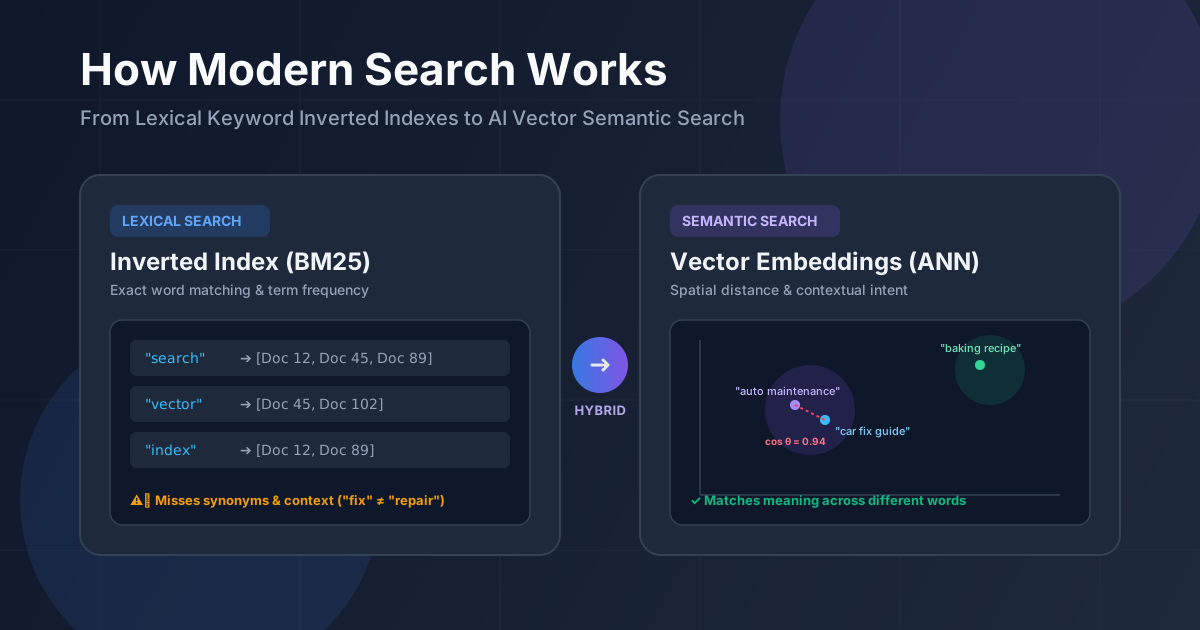
How Modern Search Works: A Practical Guide from Keywords to Semantic Search

Explore how search engines evolved from exact keyword matching to understanding human intent through vector embeddings, approximate nearest neighbor indexes, and hybrid architectures.

For decades, digital search relied on a simple premise: if a user types a word, find the documents containing that exact word. If you searched for "laptop battery replacement", the search engine looked through its index for pages containing "laptop", "battery", and "replacement".

This approach worked remarkably well for simple lookups. However, it suffered from a fundamental limitation known as the vocabulary mismatch problem. If a user searched for "notebook power fix", simple keyword matching would fail to connect it to an article titled "Laptop Battery Troubleshooting Guide", even though both address the exact same topic.

Modern search engines have fundamentally evolved. Rather than merely matching letters and characters, state-of-the-art search systems understand human concepts, intent, and context.

This guide breaks down how search technology evolved from traditional keyword indexing to modern AI-powered semantic search, vector embeddings, and production-grade hybrid retrieval systems.

Level 1: The Everyday Search Dilemma

To understand why modern search works the way it does, we first need to appreciate why traditional text search breaks down at scale.

Imagine a simple CTRL+F function in a text editor. It scans a document sequentially from start to finish, checking whether a target substring matches any sequence of characters in the file.

If your dataset consists of a single ten-page document, sequential scanning is instant. But what happens when your dataset contains ten million document files, e-commerce products, or customer support tickets?

Sequential scanning fails for two major reasons:

Performance: Scanning gigabytes of unstructured text for every user query takes seconds or minutes. At scale, runtime complexity scales linearly as $O(N)$, which is unacceptably slow for interactive search.
Semantics: Computers treat text as arbitrary bytes. To a basic string matcher, "car" and "automobile" are as completely unrelated as "car" and "refrigerator".

Solving the performance issue required inverted indexes. Solving the semantic issue required vector embeddings.

Level 2: Classic Keyword Search (Lexical Search)

Traditional search engines, such as Elasticsearch, Apache Lucene, and PostgreSQL full-text search, rely on Lexical Search. Lexical search relies on an ingenious data structure: the Inverted Index.

The Inverted Index

Think of a physical textbook. At the back of the book, an index lists key terms alphabetically alongside the specific page numbers where those terms appear.

An inverted index works the exact same way for digital documents. Instead of mapping a document ID to its content, an inverted index maps individual words (tokens) to a list of document IDs (known as a posting list) where those words occur.

Before text enters an inverted index, it passes through a text processing pipeline:

Tokenization: Breaking raw text strings into individual words or tokens.
Lowercasing: Converting all text to lowercase so "Search" and "search" match.
Stop-word removal: Filtering out ultra-common words that carry little predictive meaning, such as "the", "is", and "at".
Stemming and Lemmatization: Reducing words to their root forms (for instance, converting "running", "runs", and "ran" to their base root "run").

Here is a simplified visual representation contrasting how raw documents are stored versus how an inverted index organizes terms:

{
  "documents": [
    { "id": 1, "text": "Engineers build scalable search engines." },
    { "id": 2, "text": "Search algorithms index text documents efficiently." }
  ],
  "inverted_index": {
    "algorithm": [2],
    "build": [1],
    "document": [2],
    "efficiently": [2],
    "engineer": [1],
    "engine": [1],
    "index": [2],
    "scalable": [1],
    "search": [1, 2]
  }
}

When a user searches for "scalable search", the engine does not scan the full text of Document 1 or Document 2. It simply performs a hash lookup on the tokens "scalable" (Document 1) and "search" (Documents 1 and 2), identifying matching candidates instantly.

Relevance Scoring: From TF-IDF to BM25

Finding matching documents is only half the battle. A search engine must also rank those documents so the most relevant results appear at the top.

Early relevance scoring used TF-IDF (Term Frequency-Inverse Document Frequency):

Term Frequency (TF): How often a word appears in a specific document. Words appearing more frequently in a document are assumed to be more relevant to that document.
Inverse Document Frequency (IDF): How rare a word is across the entire corpus. A rare word like "kubernetes" carries far higher search weight than a common word like "guide".

While TF-IDF was a major milestone, it suffered from two key flaws: document length bias (longer documents naturally accumulate higher word counts) and linear word frequency scaling (a document containing a word twenty times is not necessarily twenty times more relevant than one containing it five times).

Modern lexical search relies on BM25 (Best Matching 25), a probabilistic ranking function that improves upon TF-IDF in two critical ways:

Term Frequency Saturation: BM25 caps the score benefit of repeated words. Once a search term appears a few times in a document, additional occurrences yield diminishing returns.
Document Length Normalization: BM25 penalizes long, wordy documents so shorter, tightly targeted articles receive fair relevance scores.

Strengths and Weaknesses of Lexical Search

Lexical search remains vital today because it is fast, deterministic, and highly accurate for specific queries:

Strengths: Perfect for exact matches (part numbers, serial codes, product SKUs, proper names, error logs), highly memory efficient, and fully explainable.
Weaknesses: Completely blind to context, synonyms, typos, or intent. Searching for "how to fix a flat tire" will miss an article titled "Punctured Wheel Repair" if keywords do not overlap.

Level 3: The Conceptual Shift – What is a Vector Embedding?

To move beyond literal character matching, we must represent text based on its underlying meaning rather than its letters. This is accomplished using Vector Embeddings.

An embedding is a numerical representation of data (words, sentences, images, or entire documents) structured as a dense array of floating-point numbers.

The Spatial Analogy

Imagine a large two-dimensional room. We want to place different items inside this room based on two specific characteristics:

X-axis: Sweetness (from savory to sweet)
Y-axis: Crunchiness (from soft to crunchy)

If we plot several items on this grid:

An Apple would land at coordinates [0.8, 0.9] (high sweetness, high crunchiness).
A Celery stick would land at [0.1, 0.9] (low sweetness, high crunchiness).
A Banana would land at [0.85, 0.2] (high sweetness, low crunchiness).
A Donut would land at [0.9, 0.1] (high sweetness, low crunchiness).

Notice what happens naturally in this geometric space: Banana and Donut end up sitting right next to each other because they share similar structural traits on our axes, even though the words "banana" and "donut" share zero letters.

Crunchiness
  ▲
  │   [Celery]                [Apple]
  │   (0.1, 0.9)              (0.8, 0.9)
  │
  │
  │   [Soft Bread]            [Banana]     [Donut]
  │   (0.1, 0.2)              (0.85, 0.2)  (0.9, 0.1)
  └──────────────────────────────────────────────────► Sweetness

High-Dimensional Vector Spaces

Real-world language embedding models (such as OpenAI's text-embedding-3, Cohere Embed, or open-source Hugging Face transformers) do not use just two dimensions. They plot text across 768, 1536, or even 3072 dimensions.

Instead of simple human-defined traits like sweetness or crunchiness, these high-dimensional axes capture subtle, abstract concepts learned from massive text training datasets: formality, sentiment, domain category, tense, implicit subject matter, and functional intent.

In a high-dimensional vector space, concepts align mathematically. A famous illustration of this vector arithmetic in word embeddings is:

$$\text{Vector("King")} - \text{Vector("Man")} + \text{Vector("Woman")} \approx \text{Vector("Queen")}$$

When an embedding model processes text, it compresses the rich contextual meaning of a sentence into a fixed-length list of floating-point numbers:

{
  "document_text": "How to replace a flat tire on a highway",
  "vector_embedding": [
    -0.0241, 0.0812, -0.0049, 0.0351, -0.0718, 0.0194, -0.0512, 0.0934, 0.0117,
    -0.0428
    /* ... 1526 additional floating point numbers ... */
  ]
}

Level 4: How Semantic Search Works

Semantic search replaces strict word matching with spatial distance calculations.

When a user submits a search query, two things happen:

The query text passes through the exact same embedding model used to index the document collection, generating a query vector.
The search system calculates the distance between the query vector and the pre-computed document vectors stored in the database.

Distance Metrics

To measure how close two vectors sit in a multi-dimensional space, search engines use mathematical distance metrics:

Cosine Similarity: Measures the cosine of the angle between two directional arrows originating from the center of the vector space. It evaluates directional alignment rather than length, yielding a score between -1 (opposite) and 1 (identical direction).
Dot Product: Multiplies corresponding vector components and sums the results. When vectors are normalized to unit length, Dot Product matches Cosine Similarity while running significantly faster on hardware.
Euclidean Distance ($L_2$): Measures the straight-line distance between two point coordinates in space.

Cosine Similarity = (A · B) / (||A|| * ||B||)

If two vector arrows point in nearly the exact same direction in vector space, their cosine similarity approaches 1.0. This indicates that the query and document share deeply aligned conceptual meanings, even if they use completely different vocabularies.

Semantic Search Strengths and Limitations

Semantic search unlocks capabilities that lexical search could never achieve:

Synonym & Intent Awareness: Searching for "stomach ache remedy" successfully returns documents about "treating abdominal pain" without explicit mapping rules.
Cross-Lingual Retrieval: Multilingual embedding models map English, Spanish, and Japanese descriptions of the same concept to nearby points in the same shared vector space.
Robustness to Ambiguity: Natural language queries phrased as complete questions work seamlessly.

However, semantic search has distinct limitations:

Weak Exact-Match Handling: Semantic models struggle with exact identifiers such as serial codes, product IDs (SKU-99482), or obscure proper names, often treating them as generic noisy tokens.
Higher Compute Cost: Generating embeddings requires neural net inferences, and comparing floating-point arrays requires substantial GPU or CPU memory bandwidth.

Level 5: Scaling Semantic Search in Production

Calculating the cosine similarity between a query vector and every document vector in your database works fine for a tutorial with 500 documents. But what happens when you have 50 million documents?

Calculating exact vector distances against every document is known as a k-Nearest Neighbors (k-NN) brute-force scan. Because each query comparison requires $O(N)$ high-dimensional vector calculations, brute-force search quickly freezes under real-world traffic.

To serve queries in under 50 milliseconds, production systems rely on Approximate Nearest Neighbor (ANN) algorithms.

Approximate Nearest Neighbor (ANN) Indexing

ANN algorithms trade a tiny fraction of recall accuracy (perhaps missing 1-2% of the absolute closest theoretical neighbors) in exchange for exponential speedups.

The industry-standard ANN indexing structure is HNSW (Hierarchical Navigable Small World):

Think of HNSW as a multi-layered skip list constructed across a spatial graph.
The top layer contains a sparse graph connecting points far apart from each other, allowing the search engine to jump quickly across huge conceptual distances in space.
As the search descends into lower layers, the graph density increases, allowing fine-grained local navigation to locate the tightest cluster of relevant document vectors.

Layer 2 (Sparse)  :  [Point A] ──────────────────────────► [Point Z]
                         │                                    │
Layer 1 (Medium)  :  [Point A] ──────► [Point M] ─────────► [Point Z]
                         │                │                   │
Layer 0 (Dense)   :  [Point A] ─► [P1] ─► [Point M] ─► [P2] ─► [Point Z]

Using HNSW indexing, vector lookup times drop from linear $O(N)$ brute-force scans to logarithmic $O(\log N)$ graph traversals.

Modern vector databases (such as Qdrant, Pinecone, and Milvus) along with database extensions (like PostgreSQL's pgvector) implement HNSW and Product Quantization (PQ) to store and query billions of vectors efficiently.

Level 6: The Modern Gold Standard – Hybrid Search & Re-ranking

Relying exclusively on lexical search causes missing conceptual matches. Relying exclusively on semantic search causes missing exact matches for serial numbers or names.

Production search architectures at leading tech companies avoid choosing between the two. Instead, they implement Hybrid Search.

Combining Lexical and Semantic Search

Hybrid search executes both search methodologies in parallel for every query:

Lexical Branch: Runs a classic BM25 search over an inverted index to catch exact keyword hits, code snippets, product names, and specific identifiers.
Semantic Branch: Runs an ANN vector search using embeddings to retrieve contextually relevant concepts and intent-driven matches.

Reciprocal Rank Fusion (RRF)

Because BM25 outputs arbitrary relevance scores (e.g., scores like 14.2 or 3.8) while vector search outputs cosine similarity scores bounded between 0.0 and 1.0, you cannot simply add their raw scores together.

To merge results fairly, production pipelines use Reciprocal Rank Fusion (RRF). RRF evaluates the rank position of each document within both result lists rather than relying on raw metric scores:

$$\text{RRF Score}(d) = \frac{1}{k + \text{Rank}{\text{BM25}}(d)} + \frac{1}{k + \text{Rank}{\text{Vector}}(d)}$$

Where $k$ is a constant (typically set around 60). Documents that rank near the top in both keyword search and vector search receive the highest combined RRF priority.

The Re-ranking Step (Cross-Encoders)

To achieve maximum accuracy, modern search pipelines add a final refinement step called Re-ranking.

Embedding models used during vector search are Bi-Encoders: they embed the query and documents separately so document vectors can be pre-computed. This separate embedding process is fast, but it sacrifices deep interaction between query words and document words.

A Cross-Encoder (Re-ranker) takes the query string and a top candidate document, feeds them together into a specialized neural model, and calculates a highly accurate contextual alignment score.

Because cross-encoders are computationally expensive, they are only applied to the top 30 to 50 candidate results produced by the hybrid RRF stage.

Here is the full end-to-end modern hybrid search pipeline:

flowchart TD
    UserQuery[User Input Query] --> LexicalBranch[BM25 Lexical Search]
    UserQuery --> VectorBranch[Embedding Model Inference]

    VectorBranch --> ANNLookup[ANN Vector Search / HNSW]

    LexicalBranch --> CandidateList1[Top 100 Keyword Results]
    ANNLookup --> CandidateList2[Top 100 Semantic Results]

    CandidateList1 --> RRF[Reciprocal Rank Fusion - RRF]
    CandidateList2 --> RRF

    RRF --> MergedCandidates[Top 50 Merged Candidates]
    MergedCandidates --> ReRanker[Cross-Encoder Re-Ranker]
    ReRanker --> FinalRankedResults[Final Top 10 Ranked Results]

Level 7: Summary & Practical Takeaway

Search Architecture Comparison Matrix

Feature	Lexical Search (BM25)	Semantic Search (Vector)	Hybrid Search + Re-ranking
Primary Mechanism	Inverted index word matching	Spatial distance between embeddings	BM25 + Vector ANN + Cross-Encoder
Best Used For	SKUs, part numbers, exact names, logs	Natural questions, concepts, intent	Enterprise search, production RAG, e-commerce
Speed	Sub-10ms	10ms - 50ms	20ms - 100ms
Setup Complexity	Low (standard databases)	Medium (vector database or extension)	High (requires multi-stage pipeline)
Typo & Intent Handling	Poor (requires manual fuzzy rules)	Excellent (built into model)	Exceptional (best of both worlds)
Resource Costs	Low CPU / Memory	High GPU / RAM requirements	Moderate to High compute

Developer Decision Checklist

When building search features for your own applications, use this framework to choose the right strategy:

Choose Lexical Search (BM25) if your application primarily handles structured data lookups, SKU numbers, code repository identifiers, log analysis, or if infrastructure simplicity is your highest priority.
Choose Semantic Search if your users enter conversational queries, questions, or multi-lingual search terms where context and meaning matter far more than literal word matches.
Choose Hybrid Search with Re-ranking if you are building production Retrieval-Augmented Generation (RAG) applications, enterprise knowledge bases, or e-commerce search platforms where missing an exact part number is just as bad as missing a broad conceptual answer.

By understanding how inverted indexes, vector spaces, ANN graphs, and re-rankers fit together, you can design search systems that deliver fast, intuitive, and remarkably accurate answers to your users.